This is part of a series:
- Exploratory Data Analysis – House Prices – Part 1
- Exploratory Data Analysis – House Prices – Part 2
- Data Science Project: Data Cleaning Script – House Prices DataSet
- Data Science Project: Machine Learning Model – House Prices Dataset
- Data Science Project: House Prices Dataset – API
- Data Science and Machine Learning Project: House Prices Dataset
In this article we are going to do an Exploratory Data Analysis, a.k.a EDA, of the dataset "House Prices: Advanced Regression Techniques".
In this Part 1 we will:
- Understand the problem
- Explore the data and deal with missing values
In Part 2 we will:
- Prepare the data
- Select and transform variables, especially categorical ones
The Problem
This is the description of the problem on Kaggle:
"Ask a home buyer to describe their dream house, and they probably won’t begin with the height of the basement ceiling or the proximity to an east-west railroad. But this playground competition’s dataset proves that much more influences price negotiations than the number of bedrooms or a white-picket fence.
With 79 explanatory variables describing (almost) every aspect of residential homes in Ames, Iowa, this competition challenges you to predict the final price of each home."
So, we are going to explore the dataset, try to get some insights from it, and use some tools to transform the data into formats that make more sense.
Initial Exploration and First Insights
In this section, we are going to make an initial exploration of the dataset.
This EDA was performed on a Jupyter Notebook and you can download the notebook of this part 1 of the EDA, but the notebook is more raw and don’t have the explanations.
Importing Libraries
We begin by importing the libs we are going to use:
- The standard math module provides access to the mathematical functions.
- The NumPy lib is fundamental for any kind of scientific computing with Python.
- pandas is a must-have tool for data analysis and manipulation.
- matplotlib is the most complete package in Python when it comes to data visualizations.
- seaborn is based on matplotlib as a higher-level set of visualization tools, not as powerful as matplotlib, but much easier to work with and delivers a lot with less work.
import math
import numpy as np
import pandas as pd
import seaborn as sns
import matplotlib as mpl
import matplotlib.pyplot as plt

%matplotlib inline
Loading Data
Since we have tabular data, we are going to use pandas to load the data and take a first look at it.
To load the data, since the format is CSV (Comma-Separated Values), we use the read_csv() function from pandas.
Then we print its shape, which is 1168×81, meaning we have 1168 rows (records) and 81 columns (features).
Actually, we have 1169 rows in the CSV file, but the header that describes the columns doesn’t count.
And we actually have 79 features since one of the columns is SalePrice, which is the column we will try to predict in a model, and we also will not use the column Id and will get rid of it later.
The dataset can be downloaded from Homes Dataset.
train = pd.read_csv('../data/raw/train.csv')
train.shape
(1168, 81)Looking at the Data
First, I recommend you to read this brief description of each column.
Using the head() function from pandas with an argument of 3, we can take a look at the first 3 records.
The .T means Transpose, this way we visualize rows as columns and vice-versa.
Notice how it doesn’t show all of the columns in the middle and only displays ... because there are too many of them.
train.head(3).T| 0 | 1 | 2 | |
|---|---|---|---|
| Id | 893 | 1106 | 414 |
| MSSubClass | 20 | 60 | 30 |
| MSZoning | RL | RL | RM |
| LotFrontage | 70 | 98 | 56 |
| LotArea | 8414 | 12256 | 8960 |
| … | … | … | … |
| MoSold | 2 | 4 | 3 |
| YrSold | 2006 | 2010 | 2010 |
| SaleType | WD | WD | WD |
| SaleCondition | Normal | Normal | Normal |
| SalePrice | 154500 | 325000 | 115000 |
81 rows × 3 columns
The info() method from pandas will give you a summary of the data.
Notice how Alley has 70 non-null values, meaning it doesn’t have a value for most of the 1168 records.
We can also visualize the data types.
train.info()
RangeIndex: 1168 entries, 0 to 1167
Data columns (total 81 columns):
Id               1168 non-null int64
MSSubClass       1168 non-null int64
MSZoning         1168 non-null object
LotFrontage      964 non-null float64
LotArea          1168 non-null int64
Street           1168 non-null object
Alley            70 non-null object
LotShape         1168 non-null object
LandContour      1168 non-null object
Utilities        1168 non-null object
LotConfig        1168 non-null object
LandSlope        1168 non-null object
Neighborhood     1168 non-null object
Condition1       1168 non-null object
Condition2       1168 non-null object
BldgType         1168 non-null object
HouseStyle       1168 non-null object
OverallQual      1168 non-null int64
OverallCond      1168 non-null int64
YearBuilt        1168 non-null int64
YearRemodAdd     1168 non-null int64
RoofStyle        1168 non-null object
RoofMatl         1168 non-null object
Exterior1st      1168 non-null object
Exterior2nd      1168 non-null object
MasVnrType       1160 non-null object
MasVnrArea       1160 non-null float64
ExterQual        1168 non-null object
ExterCond        1168 non-null object
Foundation       1168 non-null object
BsmtQual         1138 non-null object
BsmtCond         1138 non-null object
BsmtExposure     1137 non-null object
BsmtFinType1     1138 non-null object
BsmtFinSF1       1168 non-null int64
BsmtFinType2     1137 non-null object
BsmtFinSF2       1168 non-null int64
BsmtUnfSF        1168 non-null int64
TotalBsmtSF      1168 non-null int64
Heating          1168 non-null object
HeatingQC        1168 non-null object
CentralAir       1168 non-null object
Electrical       1167 non-null object
1stFlrSF         1168 non-null int64
2ndFlrSF         1168 non-null int64
LowQualFinSF     1168 non-null int64
GrLivArea        1168 non-null int64
BsmtFullBath     1168 non-null int64
BsmtHalfBath     1168 non-null int64
FullBath         1168 non-null int64
HalfBath         1168 non-null int64
BedroomAbvGr     1168 non-null int64
KitchenAbvGr     1168 non-null int64
KitchenQual      1168 non-null object
TotRmsAbvGrd     1168 non-null int64
Functional       1168 non-null object
Fireplaces       1168 non-null int64
FireplaceQu      617 non-null object
GarageType       1099 non-null object
GarageYrBlt      1099 non-null float64
GarageFinish     1099 non-null object
GarageCars       1168 non-null int64
GarageArea       1168 non-null int64
GarageQual       1099 non-null object
GarageCond       1099 non-null object
PavedDrive       1168 non-null object
WoodDeckSF       1168 non-null int64
OpenPorchSF      1168 non-null int64
EnclosedPorch    1168 non-null int64
3SsnPorch        1168 non-null int64
ScreenPorch      1168 non-null int64
PoolArea         1168 non-null int64
PoolQC           4 non-null object
Fence            217 non-null object
MiscFeature      39 non-null object
MiscVal          1168 non-null int64
MoSold           1168 non-null int64
YrSold           1168 non-null int64
SaleType         1168 non-null object
SaleCondition    1168 non-null object
SalePrice        1168 non-null int64
dtypes: float64(3), int64(35), object(43)
memory usage: 739.2+ KB
The describe() method is good to have the first insights of the data.
It automatically gives you descriptive statistics for each feature: number of non-NA/null observations, mean, standard deviation, the min value, the quartiles, and the max value.
Note that the calculations don’t take NaN values into consideration.
For LotFrontage, for instance, it uses only the 964 non-null values, and excludes the other 204 null observations.
train.describe().T| count | mean | std | min | 25% | 50% | 75% | max | |
|---|---|---|---|---|---|---|---|---|
| Id | 1168.0 | 720.240582 | 420.237685 | 1.0 | 355.75 | 716.5 | 1080.25 | 1460.0 |
| MSSubClass | 1168.0 | 56.699486 | 41.814065 | 20.0 | 20.00 | 50.0 | 70.00 | 190.0 |
| LotFrontage | 964.0 | 70.271784 | 25.019386 | 21.0 | 59.00 | 69.5 | 80.00 | 313.0 |
| LotArea | 1168.0 | 10597.720890 | 10684.958323 | 1477.0 | 7560.00 | 9463.0 | 11601.50 | 215245.0 |
| OverallQual | 1168.0 | 6.095034 | 1.403402 | 1.0 | 5.00 | 6.0 | 7.00 | 10.0 |
| OverallCond | 1168.0 | 5.594178 | 1.116842 | 1.0 | 5.00 | 5.0 | 6.00 | 9.0 |
| YearBuilt | 1168.0 | 1971.120719 | 30.279560 | 1872.0 | 1954.00 | 1972.0 | 2000.00 | 2009.0 |
| YearRemodAdd | 1168.0 | 1985.200342 | 20.498566 | 1950.0 | 1968.00 | 1994.0 | 2004.00 | 2010.0 |
| MasVnrArea | 1160.0 | 104.620690 | 183.996031 | 0.0 | 0.00 | 0.0 | 166.25 | 1600.0 |
| BsmtFinSF1 | 1168.0 | 444.345890 | 466.278751 | 0.0 | 0.00 | 384.0 | 706.50 | 5644.0 |
| BsmtFinSF2 | 1168.0 | 46.869863 | 162.324086 | 0.0 | 0.00 | 0.0 | 0.00 | 1474.0 |
| BsmtUnfSF | 1168.0 | 562.949486 | 445.605458 | 0.0 | 216.00 | 464.5 | 808.50 | 2336.0 |
| TotalBsmtSF | 1168.0 | 1054.165240 | 448.848911 | 0.0 | 792.75 | 984.0 | 1299.00 | 6110.0 |
| 1stFlrSF | 1168.0 | 1161.268836 | 393.541120 | 334.0 | 873.50 | 1079.5 | 1392.00 | 4692.0 |
| 2ndFlrSF | 1168.0 | 351.218322 | 437.334802 | 0.0 | 0.00 | 0.0 | 730.50 | 2065.0 |
| LowQualFinSF | 1168.0 | 5.653253 | 48.068312 | 0.0 | 0.00 | 0.0 | 0.00 | 572.0 |
| GrLivArea | 1168.0 | 1518.140411 | 534.904019 | 334.0 | 1133.25 | 1467.5 | 1775.25 | 5642.0 |
| BsmtFullBath | 1168.0 | 0.426370 | 0.523376 | 0.0 | 0.00 | 0.0 | 1.00 | 3.0 |
| BsmtHalfBath | 1168.0 | 0.061644 | 0.244146 | 0.0 | 0.00 | 0.0 | 0.00 | 2.0 |
| FullBath | 1168.0 | 1.561644 | 0.555074 | 0.0 | 1.00 | 2.0 | 2.00 | 3.0 |
| HalfBath | 1168.0 | 0.386130 | 0.504356 | 0.0 | 0.00 | 0.0 | 1.00 | 2.0 |
| BedroomAbvGr | 1168.0 | 2.865582 | 0.817491 | 0.0 | 2.00 | 3.0 | 3.00 | 8.0 |
| KitchenAbvGr | 1168.0 | 1.046233 | 0.218084 | 1.0 | 1.00 | 1.0 | 1.00 | 3.0 |
| TotRmsAbvGrd | 1168.0 | 6.532534 | 1.627412 | 2.0 | 5.00 | 6.0 | 7.00 | 14.0 |
| Fireplaces | 1168.0 | 0.612158 | 0.640872 | 0.0 | 0.00 | 1.0 | 1.00 | 3.0 |
| GarageYrBlt | 1099.0 | 1978.586897 | 24.608158 | 1900.0 | 1962.00 | 1980.0 | 2002.00 | 2010.0 |
| GarageCars | 1168.0 | 1.761130 | 0.759039 | 0.0 | 1.00 | 2.0 | 2.00 | 4.0 |
| GarageArea | 1168.0 | 473.000000 | 218.795260 | 0.0 | 318.75 | 479.5 | 577.00 | 1418.0 |
| WoodDeckSF | 1168.0 | 92.618151 | 122.796184 | 0.0 | 0.00 | 0.0 | 168.00 | 736.0 |
| OpenPorchSF | 1168.0 | 45.256849 | 64.120769 | 0.0 | 0.00 | 24.0 | 68.00 | 523.0 |
| EnclosedPorch | 1168.0 | 20.790240 | 58.308987 | 0.0 | 0.00 | 0.0 | 0.00 | 330.0 |
| 3SsnPorch | 1168.0 | 3.323630 | 27.261055 | 0.0 | 0.00 | 0.0 | 0.00 | 407.0 |
| ScreenPorch | 1168.0 | 14.023116 | 52.498520 | 0.0 | 0.00 | 0.0 | 0.00 | 410.0 |
| PoolArea | 1168.0 | 1.934075 | 33.192538 | 0.0 | 0.00 | 0.0 | 0.00 | 648.0 |
| MiscVal | 1168.0 | 42.092466 | 538.941473 | 0.0 | 0.00 | 0.0 | 0.00 | 15500.0 |
| MoSold | 1168.0 | 6.377568 | 2.727010 | 1.0 | 5.00 | 6.0 | 8.00 | 12.0 |
| YrSold | 1168.0 | 2007.815068 | 1.327339 | 2006.0 | 2007.00 | 2008.0 | 2009.00 | 2010.0 |
| SalePrice | 1168.0 | 181081.876712 | 81131.228007 | 34900.0 | 129975.00 | 162950.0 | 214000.00 | 755000.0 |
Data Cleaning
In this section, we will perform some Data Cleaning.
The id column
The id column is only a dumb identification with no correlation to SalePrice.
So let’s remove the id:
train.drop(columns=['Id'], inplace=True)Missing values
When we used info() to see the data summary, we could see many columns had a bunch of missing data.
Let’s see which columns have missing values and the proportion in each one of them.
isna() from pandas will return the missing values for each column, then the sum() function will add them up to give you a total.
columns_with_miss = train.isna().sum()
#filtering only the columns with at least 1 missing value
columns_with_miss = columns_with_miss[columns_with_miss!=0]
#The number of columns with missing values
print('Columns with missing values:', len(columns_with_miss))
#sorting the columns by the number of missing values descending
columns_with_miss.sort_values(ascending=False)
Columns with missing values: 19
PoolQC 1164
MiscFeature 1129
Alley 1098
Fence 951
FireplaceQu 551
LotFrontage 204
GarageYrBlt 69
GarageType 69
GarageFinish 69
GarageQual 69
GarageCond 69
BsmtFinType2 31
BsmtExposure 31
BsmtFinType1 30
BsmtCond 30
BsmtQual 30
MasVnrArea 8
MasVnrType 8
Electrical 1
dtype: int64Out of 80 columns, 19 have missing values.
Missing values per se it not a big problem, but columns with a high number of missing values can cause distortions.
This is the case for:
- PoolQC: Pool quality
- MiscFeature: Miscellaneous feature not covered in other categories
- Alley: Type of alley access to property
- Fence: Fence quality
Let’s drop them from the dataset for now.
# Removing columns
train.drop(columns=['PoolQC', 'MiscFeature', 'Alley', 'Fence'], inplace=True)
FireplaceQu has 551 missing values, which is also pretty high.
In this case, the missing values have meaning, which is "NO Fireplace".
Fireplace has the following categories:
- Ex Excellent – Exceptional Masonry Fireplace
- Gd Good – Masonry Fireplace in main level
- TA Average – Prefabricated Fireplace in main living area or Masonry Fireplace in basement
- Fa Fair – Prefabricated Fireplace in basement
- Po Poor – Ben Franklin Stove
- NA No Fireplace
Let’s check the correlation between FireplaceQu and SalePrice, to see how important this feature is in order to determine the price.
First, we will replace the missing values for 0.
Then, we encode the categories into numbers from 1 to 5.
train['FireplaceQu'].fillna(0, inplace=True)
train['FireplaceQu'].replace({'Po': 1, 'Fa': 2, 'TA': 3, 'Gd': 4, 'Ex': 5}, inplace=True)
Using a barplot, we can see how the category of the FirePlace increases the value of SalePrice.
It is also worth noting how much higher the value is when the house has an Excellent fireplace.
This means we should keep FireplaceQu as feature.
sns.set(style="whitegrid")
sns.barplot(x='FireplaceQu', y="SalePrice", data=train)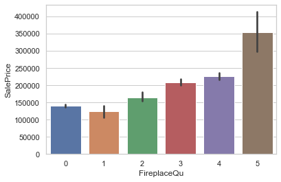
Missing values in numeric columns
Another feature with a high number of missing values is LotFrontage with a count 204.
Let’s see the correlation between the remaining features with missing values and the SalePrice.
columns_with_miss = train.isna().sum()
columns_with_miss = columns_with_miss[columns_with_miss!=0]
c = list(columns_with_miss.index)
c.append('SalePrice')
train[c].corr()| LotFrontage | MasVnrArea | GarageYrBlt | SalePrice | |
|---|---|---|---|---|
| LotFrontage | 1.000000 | 0.196649 | 0.089542 | 0.371839 |
| MasVnrArea | 0.196649 | 1.000000 | 0.253348 | 0.478724 |
| GarageYrBlt | 0.089542 | 0.253348 | 1.000000 | 0.496575 |
| SalePrice | 0.371839 | 0.478724 | 0.496575 | 1.000000 |
Note that LotFrontage, MasVnrArea, and GarageYrBlt have a positive correlation with SalePrice, but this correlation isn’t very strong.
To simplify this analisys, we will remove theses columns for now:
cols_to_be_removed = ['LotFrontage', 'GarageYrBlt', 'MasVnrArea']
train.drop(columns=cols_to_be_removed, inplace=True)
Finally, these are the remaining columns with missing values:
columns_with_miss = train.isna().sum()
columns_with_miss = columns_with_miss[columns_with_miss!=0]
print(f'Columns with missing values: {len(columns_with_miss)}')
columns_with_miss.sort_values(ascending=False)
Columns with missing values: 11
GarageCond 69
GarageQual 69
GarageFinish 69
GarageType 69
BsmtFinType2 31
BsmtExposure 31
BsmtFinType1 30
BsmtCond 30
BsmtQual 30
MasVnrType 8
Electrical 1
dtype: int64Conclusion
In this part 1 we dealt with missing values and removed the following columns: ‘Id’, ‘PoolQC’, ‘MiscFeature’, ‘Alley’, ‘Fence’, ‘LotFrontage’, ‘GarageYrBlt’, ‘MasVnrArea’.
Please note that the removed columns are not useless or may not contribute to the final model.
After the first round of analysis and testing of the hypothesis, if you ever need to improve your future model further, you can consider reevaluating these columns and understand them better to see how they fit into the problem.
Data Analysis and Machine Learning is NOT a straight path.
It is a process where you iterate and keep testing ideas until you have the result you want, or until find out the result you need is not possible.
In Part 2 (the final part of the EDA) we will see ways to handle the missing values in the other 11 columns.
We will also explore categorical variables.