This is part of a series:
- Exploratory Data Analysis – House Prices – Part 1
- Exploratory Data Analysis – House Prices – Part 2
- Data Science Project: Data Cleaning Script – House Prices DataSet
- Data Science Project: Machine Learning Model – House Prices Dataset
- Data Science Project: House Prices Dataset – API
- Data Science and Machine Learning Project: House Prices Dataset
In this article, we will finish the Exploratory Data Analysis, a.k.a EDA, and cleaning of the data of the dataset House Prices: Advanced Regression Techniques.
In Part 1 we:
- Understood the problem
- Explored the data and dealt with missing values
In this post we will:
- Prepare the data
- Select and transform variables, especially categorical ones
You can download the compĺete Jupyter Notebook covering part 1 and 2 of the EDA, but the notebook is just code and don’t have the explanations.
The following steps are a direct continuation of the ones in Part 1.
Categorical variables
Let’s work on the categorical variables of our dataset.
Dealing with missing values
Filling Categorical NaN that we know how to fill due to the description file.
# Fills NA in place of NaN
for c in ['GarageType', 'GarageFinish', 'BsmtFinType2', 'BsmtExposure', 'BsmtFinType1']:
    train[c].fillna('NA', inplace=True)

# Fills None in place of NaN
train['MasVnrType'].fillna('None', inplace=True)
With this have only 5 columns with missing values left in our dataset.
columns_with_miss = train.isna().sum()
columns_with_miss = columns_with_miss[columns_with_miss!=0]
print(f'Columns with missing values: {len(columns_with_miss)}')
columns_with_miss.sort_values(ascending=False)
Columns with missing values: 5
GarageCond 69
GarageQual 69
BsmtCond 30
BsmtQual 30
Electrical 1
dtype: int64Ordinal
Also by reading the description file, we can identify other variables that have a similar system to FireplaceQu to categorize the quality: Poor, Good, Excellent, etc.
We are going to replicate the treatment we gave to FireplaceQu to these variables according to the following descriptions:
ExterQual: Evaluates the quality of the material on the exterior
- Ex Excellent
- Gd Good
- TA Average/Typical
- Fa Fair
- Po Poor
ExterCond: Evaluates the present condition of the material on the exterior
- Ex Excellent
- Gd Good
- TA Average/Typical
- Fa Fair
- Po Poor
BsmtQual: Evaluates the height of the basement
- Ex Excellent (100+ inches)
- Gd Good (90-99 inches)
- TA Typical (80-89 inches)
- Fa Fair (70-79 inches)
- Po Poor ( < 70 inches)
- NA No Basement
BsmtCond: Evaluates the general condition of the basement
- Ex Excellent
- Gd Good
- TA Typical – slight dampness allowed
- Fa Fair – dampness or some cracking or settling
- Po Poor – Severe cracking, settling, or wetness
- NA No Basement
HeatingQC: Heating quality and condition
- Ex Excellent
- Gd Good
- TA Average/Typical
- Fa Fair
- Po Poor
KitchenQual: Kitchen quality
- Ex Excellent
- Gd Good
- TA Average/Typical
- Fa Fair
- Po Poor
GarageQual: Garage quality
- Ex Excellent
- Gd Good
- TA Average/Typical
- Fa Fair
- Po Poor
- NA No Garage
GarageCond: Garage condition
- Ex Excellent
- Gd Good
- TA Average/Typical
- Fa Fair
- Po Poor
- NA No Garage
ord_cols = ['ExterQual', 'ExterCond', 'BsmtQual', 'BsmtCond', 'HeatingQC', 'KitchenQual', 'GarageQual', 'GarageCond']
for col in ord_cols:
    train[col].fillna(0, inplace=True)
    train[col].replace({'Po': 1, 'Fa': 2, 'TA': 3, 'Gd': 4, 'Ex': 5}, inplace=True)
Let’s now plot the correlation of these variables with SalePrice.
ord_cols = ['ExterQual', 'ExterCond', 'BsmtQual', 'BsmtCond', 'HeatingQC', 'KitchenQual', 'GarageQual', 'GarageCond']
f, axes = plt.subplots(2, 4, figsize=(15, 10), sharey=True)

for r in range(0, 2):
    for c in range(0, 4):
        sns.barplot(x=ord_cols.pop(), y="SalePrice", data=train, ax=axes[r][c])

plt.tight_layout()
plt.show()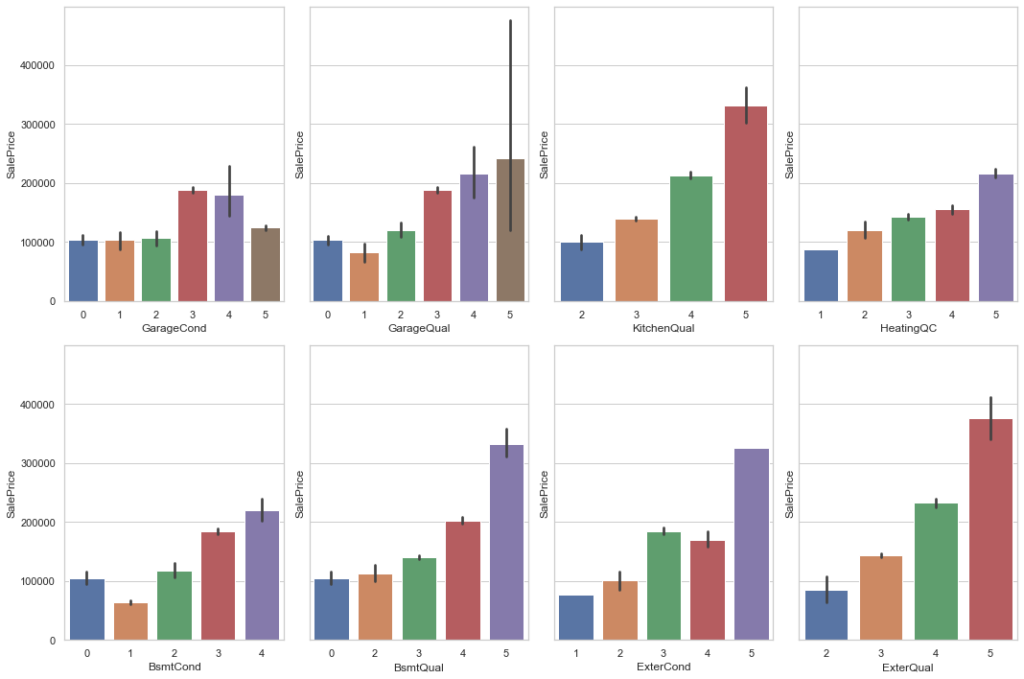
As you can see, the better the category of a variable, the higher the price, which means these variables will be important for a prediction model.
Nominal
Other categorical variables don’t seem to follow any clear ordering.
Let’s see how many values these columns can assume:
cols = train.columns
num_cols = train._get_numeric_data().columns
nom_cols = list(set(cols) - set(num_cols))
print(f'Nominal columns: {len(nom_cols)}')

value_counts = {}
for c in nom_cols:
    value_counts[c] = len(train[c].value_counts())

sorted_value_counts = {k: v for k, v in sorted(value_counts.items(), key=lambda item: item[1])}
sorted_value_counts
Nominal columns: 31
{'CentralAir': 2,
'Street': 2,
'Utilities': 2,
'LandSlope': 3,
'PavedDrive': 3,
'MasVnrType': 4,
'GarageFinish': 4,
'LotShape': 4,
'LandContour': 4,
'BsmtCond': 5,
'MSZoning': 5,
'Electrical': 5,
'Heating': 5,
'BldgType': 5,
'BsmtExposure': 5,
'LotConfig': 5,
'Foundation': 6,
'RoofStyle': 6,
'SaleCondition': 6,
'BsmtFinType2': 7,
'Functional': 7,
'GarageType': 7,
'BsmtFinType1': 7,
'RoofMatl': 7,
'HouseStyle': 8,
'Condition2': 8,
'SaleType': 9,
'Condition1': 9,
'Exterior1st': 15,
'Exterior2nd': 16,
'Neighborhood': 25}Some categorical variables can assume several different values like Neighborhood.
To simplify, let’s analyze only variables with 6 different values or less.
nom_cols_less_than_6 = []
for c in nom_cols:
    n_values = len(train[c].value_counts())
    if n_values < 7:
        nom_cols_less_than_6.append(c)

print(f'Nominal columns with less than 6 values: {len(nom_cols_less_than_6)}')
Nominal columns with less than 6 values: 19Plotting against SalePrice to have a better idea of how they affect it:
ncols = 3
nrows = math.ceil(len(nom_cols_less_than_6) / ncols)
f, axes = plt.subplots(nrows, ncols, figsize=(15, 30))

for r in range(0, nrows):
    for c in range(0, ncols):
        if not nom_cols_less_than_6:
            continue
        sns.barplot(x=nom_cols_less_than_6.pop(), y="SalePrice", data=train, ax=axes[r][c])

plt.tight_layout()
plt.show()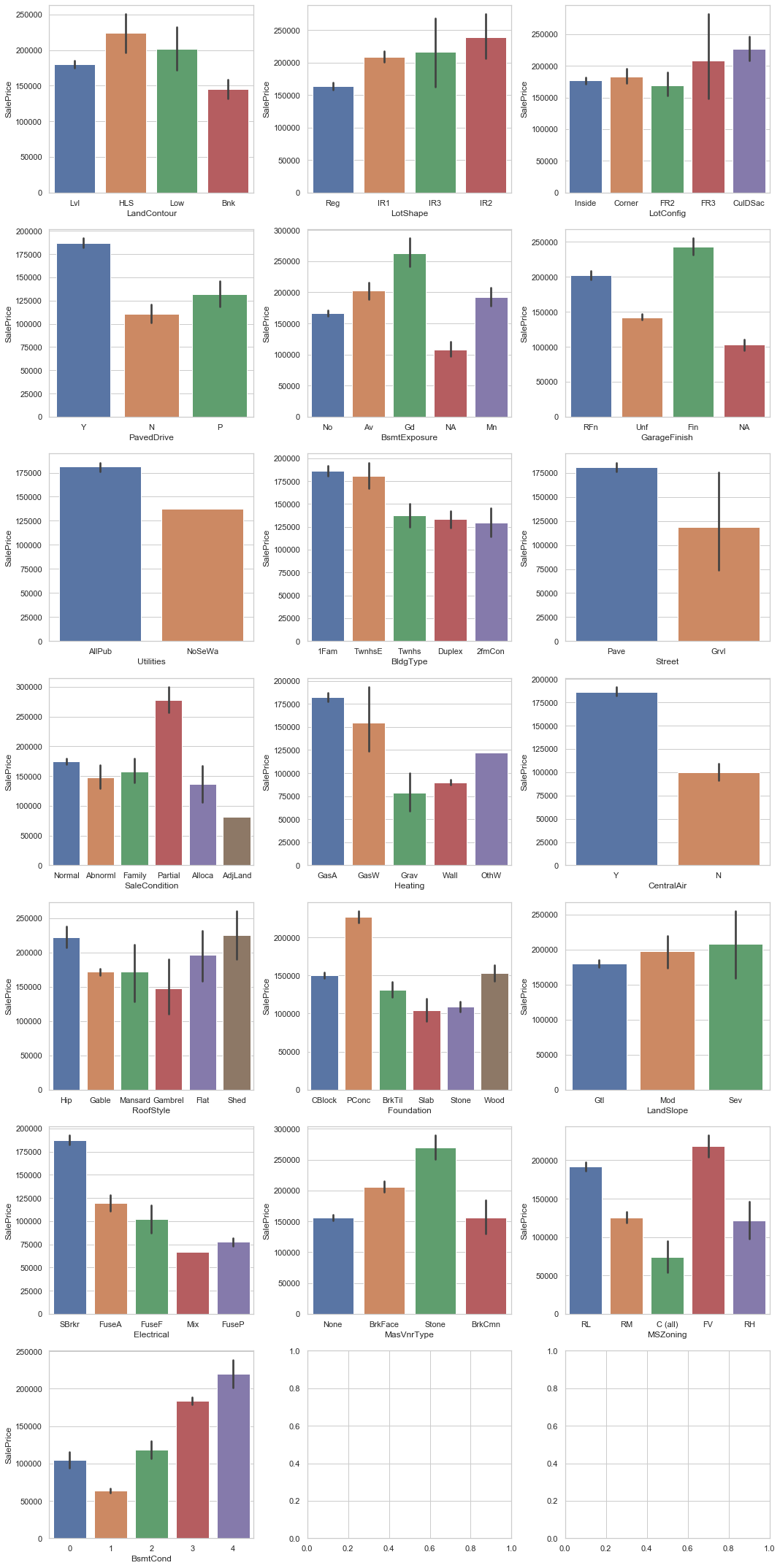
We can see a good correlation of many of these columns with the target variable.
For now, let’s keep them.
We still have NaN in ‘Electrical’.
As we could see in the plot above, ‘SBrkr’ is the most frequent value in ‘Electrical’.
Let’s use this value to replace NaN in Electrical.
# Inputs more frequent value in place of NaN

train['Electrical'].fillna('SBrkr', inplace=True)
Zero values
Another quick check is to see how many columns have lots of data equals to 0.
train.isin([0]).sum().sort_values(ascending=False).head(25)PoolArea 1164
LowQualFinSF 1148
3SsnPorch 1148
MiscVal 1131
BsmtHalfBath 1097
ScreenPorch 1079
BsmtFinSF2 1033
EnclosedPorch 1007
HalfBath 727
BsmtFullBath 686
2ndFlrSF 655
WoodDeckSF 610
Fireplaces 551
FireplaceQu 551
OpenPorchSF 534
BsmtFinSF1 382
BsmtUnfSF 98
GarageCars 69
GarageArea 69
GarageCond 69
GarageQual 69
TotalBsmtSF 30
BsmtCond 30
BsmtQual 30
FullBath 8
dtype: int64In this case, even though there are many 0’s, they have meaning.
For instance, PoolArea (Pool area in square feet) equals 0 means that the house doesn’t have any pool area.
This is important information correlated to the house and thus, we are going to keep them.
Outliers
We can also take a look at the outliers in the numeric variables.
# Get only numerical columns
numerical_columns = list(train.dtypes[train.dtypes == 'int64'].index)
len(numerical_columns)42# Create the plot grid
rows = 7
columns = 6
fig, axes = plt.subplots(rows,columns, figsize=(30,30))
x, y = 0, 0
for i, column in enumerate(numerical_columns):
sns.boxplot(x=train[column], ax=axes[x, y])
if y < columns-1:
y += 1
elif y == columns-1:
x += 1
y = 0
else:
y += 1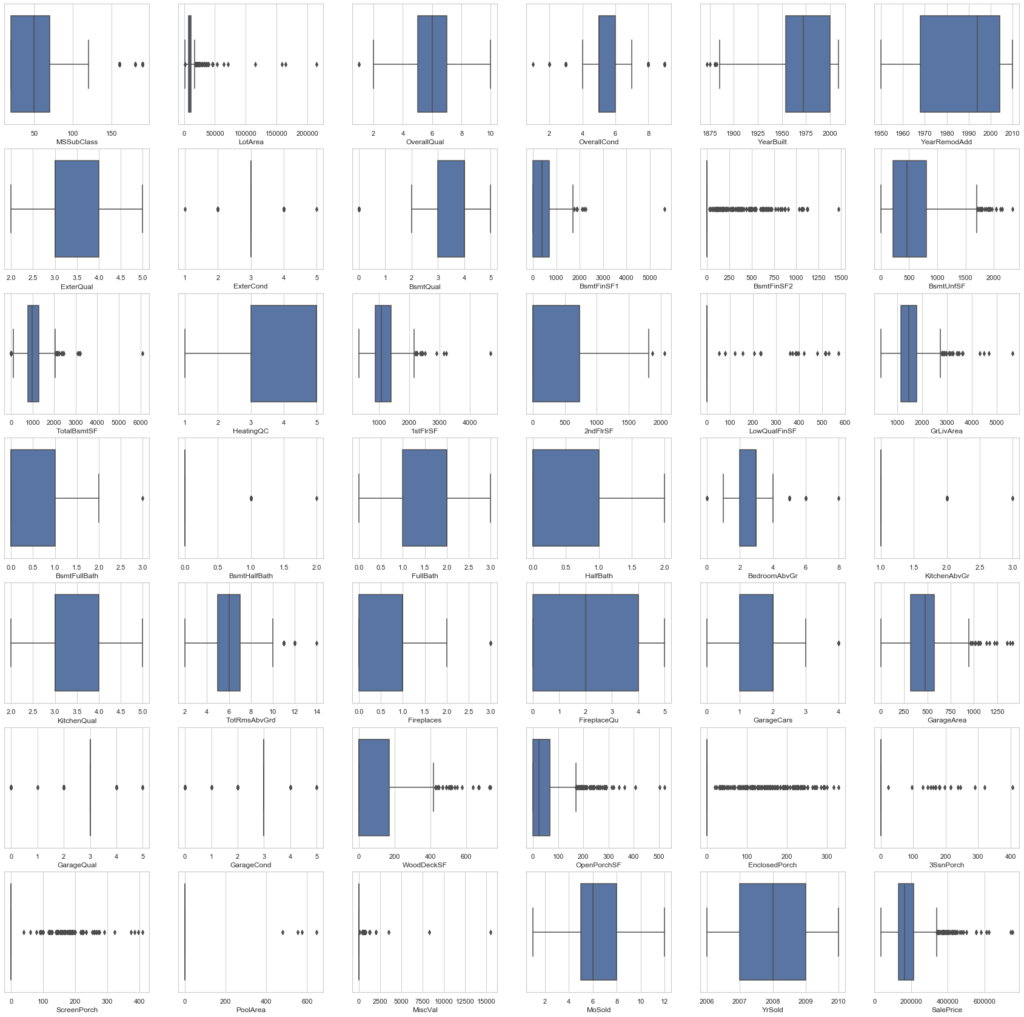
There are a lot of outliers in the dataset.
But, if we check the data description file, we see that, actually, some numerical variables, are categorical variables that were saved (codified) as numbers.
So, some of these data points that seem to be outliers are, actually, categorical data with only one example of some category.
Let’s keep these outliers.
Saving cleaned data
Let’s see how the cleaned data looks like and how many columns we have left.
We have no more missing values:
columns_with_miss = train.isna().sum()
columns_with_miss = columns_with_miss[columns_with_miss!=0]
print(f'Columns with missing values: {len(columns_with_miss)}')
columns_with_miss.sort_values(ascending=False)
Columns with missing values: 0
Series([], dtype: int64)After cleaning the data, we are left with 73 columns out of the initial 81.
train.shape(1168, 73)Let’s take a look at the first 3 records of the cleaned data.
train.head(3).T| 0 | 1 | 2 | |
|---|---|---|---|
| MSSubClass | 20 | 60 | 30 |
| MSZoning | RL | RL | RM |
| LotArea | 8414 | 12256 | 8960 |
| Street | Pave | Pave | Pave |
| LotShape | Reg | IR1 | Reg |
| … | … | … | … |
| MoSold | 2 | 4 | 3 |
| YrSold | 2006 | 2010 | 2010 |
| SaleType | WD | WD | WD |
| SaleCondition | Normal | Normal | Normal |
| SalePrice | 154500 | 325000 | 115000 |
73 rows × 3 columns
We can see a summary of the data showing that, for all the 1168 records, there isn’t a single missing (null) value.
train.info()
RangeIndex: 1168 entries, 0 to 1167
Data columns (total 73 columns):
MSSubClass       1168 non-null int64
MSZoning         1168 non-null object
LotArea          1168 non-null int64
Street           1168 non-null object
LotShape         1168 non-null object
LandContour      1168 non-null object
Utilities        1168 non-null object
LotConfig        1168 non-null object
LandSlope        1168 non-null object
Neighborhood     1168 non-null object
Condition1       1168 non-null object
Condition2       1168 non-null object
BldgType         1168 non-null object
HouseStyle       1168 non-null object
OverallQual      1168 non-null int64
OverallCond      1168 non-null int64
YearBuilt        1168 non-null int64
YearRemodAdd     1168 non-null int64
RoofStyle        1168 non-null object
RoofMatl         1168 non-null object
Exterior1st      1168 non-null object
Exterior2nd      1168 non-null object
MasVnrType       1168 non-null object
ExterQual        1168 non-null int64
ExterCond        1168 non-null int64
Foundation       1168 non-null object
BsmtQual         1168 non-null int64
BsmtCond         1168 non-null object
BsmtExposure     1168 non-null object
BsmtFinType1     1168 non-null object
BsmtFinSF1       1168 non-null int64
BsmtFinType2     1168 non-null object
BsmtFinSF2       1168 non-null int64
BsmtUnfSF        1168 non-null int64
TotalBsmtSF      1168 non-null int64
Heating          1168 non-null object
HeatingQC        1168 non-null int64
CentralAir       1168 non-null object
Electrical       1168 non-null object
1stFlrSF         1168 non-null int64
2ndFlrSF         1168 non-null int64
LowQualFinSF     1168 non-null int64
GrLivArea        1168 non-null int64
BsmtFullBath     1168 non-null int64
BsmtHalfBath     1168 non-null int64
FullBath         1168 non-null int64
HalfBath         1168 non-null int64
BedroomAbvGr     1168 non-null int64
KitchenAbvGr     1168 non-null int64
KitchenQual      1168 non-null int64
TotRmsAbvGrd     1168 non-null int64
Functional       1168 non-null object
Fireplaces       1168 non-null int64
FireplaceQu      1168 non-null int64
GarageType       1168 non-null object
GarageFinish     1168 non-null object
GarageCars       1168 non-null int64
GarageArea       1168 non-null int64
GarageQual       1168 non-null int64
GarageCond       1168 non-null int64
PavedDrive       1168 non-null object
WoodDeckSF       1168 non-null int64
OpenPorchSF      1168 non-null int64
EnclosedPorch    1168 non-null int64
3SsnPorch        1168 non-null int64
ScreenPorch      1168 non-null int64
PoolArea         1168 non-null int64
MiscVal          1168 non-null int64
MoSold           1168 non-null int64
YrSold           1168 non-null int64
SaleType         1168 non-null object
SaleCondition    1168 non-null object
SalePrice        1168 non-null int64
dtypes: int64(42), object(31)
memory usage: 666.2+ KB
Finally, let’s save the cleaned data in a separate file.
train.to_csv('train-cleaned.csv')Conclusions
In Part 1 we dealt with missing values and removed the following columns: ‘Id’, ‘PoolQC’, ‘MiscFeature’, ‘Alley’, ‘Fence’, ‘LotFrontage’, ‘GarageYrBlt’, ‘MasVnrArea’.
In this Part 2 we:
Replaced the NaN with NA in the following columns: ‘GarageType’, ‘GarageFinish’, ‘BsmtFinType2’, ‘BsmtExposure’, ‘BsmtFinType1’.
Replaced the NaN with None in ‘MasVnrType’.
Imputed the most frequent value in place of NaN in ‘Electrical’.
We are going to use this data to create our Machine Learning model and predict the house prices in the next post of this series.
Remember you can download the compĺete Jupyter Notebook covering part 1 and 2 of the EDA, but the notebook is just code and don’t have the explanations.